[1] 100This vignette introduces the micromort package, which provides tools for understanding and visualizing risks.
1. Micromorts (Acute Risk)
A micromort is a unit of risk representing a one-in-a-million chance of death. More precisely, it’s a microprobability of death — a one-in-a-million chance of a specific event (death) occurring.
Definition
| Term | Definition | Example |
|---|---|---|
| Microprobability | 1-in-a-million chance of any event | 1 micromort = microprobability of death |
| Micromort | 1-in-a-million chance of death, per event | Skydiving: 8 micromorts per jump |
Comparing Risks: Period Matters!
CRITICAL: When comparing micromort values, ensure the period is the same. For example:
| Activity | Micromorts | Period | Comparable? |
|---|---|---|---|
| Scuba diving | 5 | per dive | Per-event |
| Scuba diving | 164 | per year | Per-year (assumes ~33 dives/year) |
| Skydiving | 8 | per jump | Per-event |
The “per year” figure (164) conflates frequency with risk-per-event. A diver doing 5 dives/year vs 50 dives/year faces very different annual risk.
Conditional Risks
Many activities have selection effects. For example:
- Marathon running (7 micromorts): Runners are self-selected for fitness. This low figure reflects the health of participants, not the risk to an average person attempting a marathon.
- Motorcycle riding (10 micromorts/60 miles): Experienced riders face lower risk than novices, but the quoted figure is an average.
These figures answer: “Given that someone completed this activity, what was their death risk?” Not: “What would happen if a random person attempted this?”
Converting Probabilities to Micromorts
Common Risks Table
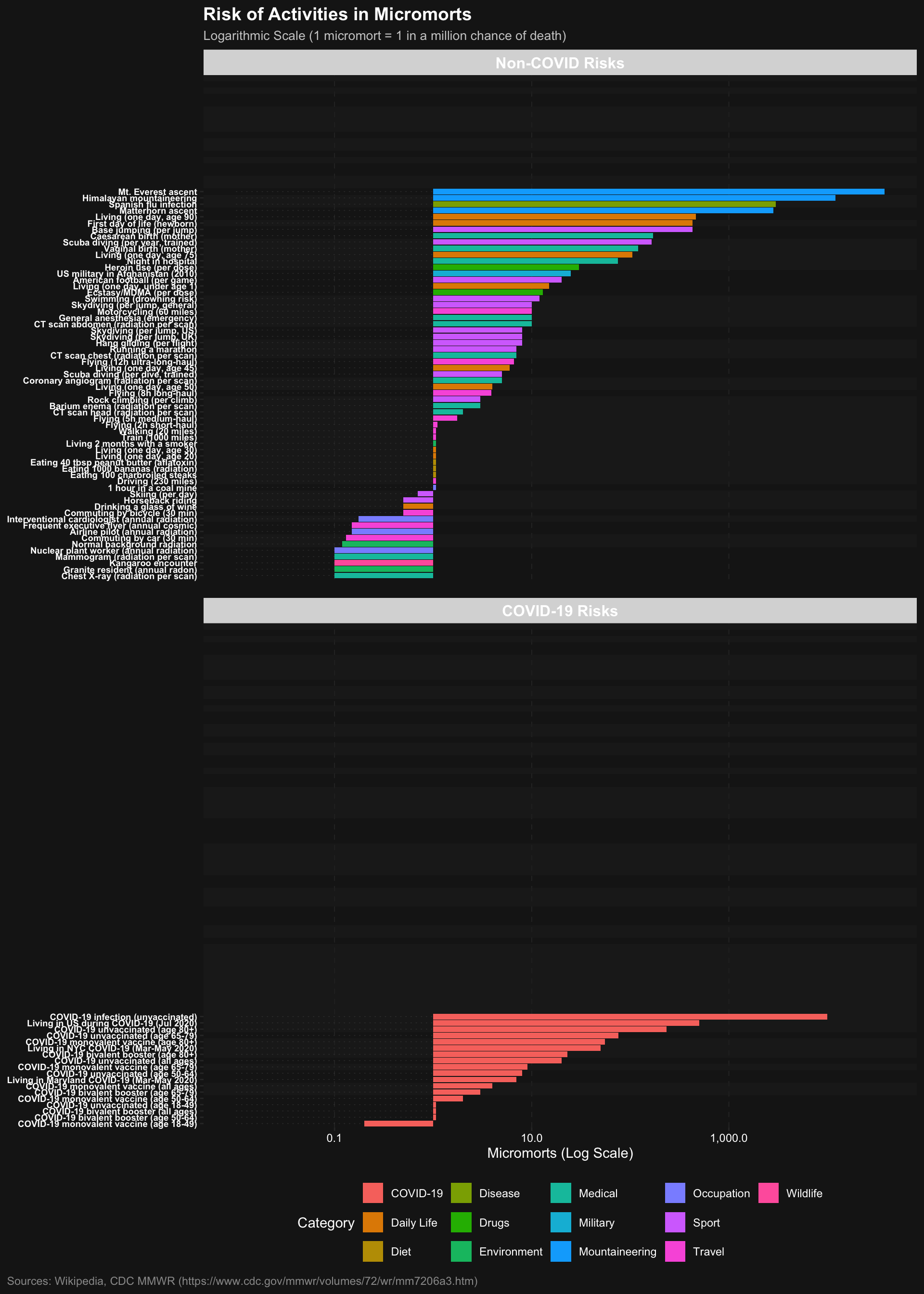
Visualizing Risks
Using plot_risks(), we can see the relative magnitude of different activities on a logarithmic scale. The plot is split into COVID-19 and Other risks to make comparisons easier:
Interactive Version
For interactive exploration with hover details and category filtering, use plot_risks_interactive():
2. Microlives (Chronic Risk)
While micromorts measure sudden death, microlives measure the impact of chronic habits on your life expectancy. A microlife represents a 30-minute change in life expectancy per day of exposure.
Living at Different Speeds
A useful way to think about microlives: we all “use up” 48 microlives per day just by living (24 hours = 48 × 30 minutes). Unhealthy habits accelerate this consumption, while healthy habits slow it down.
A smoker who smokes 20 cigarettes per day uses up an additional 10 microlives, which can be interpreted as rushing towards death at 29 hours per day instead of 24. Conversely, someone with excellent lifestyle habits might effectively live at only 22 hours per day.
Healthcare bonus: Modern healthcare and healthier lifestyles give us a “payback” of approximately 12 microlives per day — our expected death is moving away from us even as we age.
Common Chronic Risks
| Factor | Microlives/day | Interpretation |
|---|---|---|
| Smoking 1 cigarette | -1 | Lose 30 min life expectancy |
| Being 5kg overweight | -1 | Lose 30 min/day |
| 20 min moderate exercise | +2 | Gain 60 min life expectancy |
| 2+ hours TV daily | -1 | Sedentary behavior |
| 5+ servings fruit/veg | +2 | Healthy diet |
Converting Life Expectancy to Microlives
Heavy smoker (20/day): -20 microlives/day (life lost)
Moderate exercise: 2 microlives/day (life gained)
5kg overweight: -1 microlife/day (life lost)
3. Relationship Between Micromorts and Microlives
Theoretical Conversion
Micromorts (acute, per-event risk) and microlives (chronic, per-day attrition) measure different phenomena, but can be approximately converted using expected value theory.
Key relationship: 1 micromort ≈ 0.7 microlives
Assumptions for this conversion: 1. Remaining life expectancy = 40 years (use lle(prob, life_expectancy = ...) to adjust for any age; see also daily_hazard_rate()) 2. Death occurs immediately upon the event (worst case) 3. Linear approximation (valid for small probabilities)
Mathematical derivation:
- 1 micromort = 1/1,000,000 probability of death
- Expected life lost = probability × remaining life
- = 1e-6 × 40 years = 4e-5 years
- = 4e-5 × 525,960 minutes/year ≈ 21 minutes
- 1 microlife = 30 minutes, so 21 minutes ≈ 0.7 microlives
Why common_risks() uses microlives = micromorts × 0.7:
The conversion allows comparing a single risky event (like one skydive at 8 micromorts) to chronic daily habits (like smoking at -10 microlives/day). However, the approximation breaks down when:
- Remaining life expectancy differs from 40 years (a 20-year-old loses more per micromort than an 80-year-old)
- The risk is not immediate death (injuries, disabilities are not captured)
- Repeated exposures compound non-linearly
Unit Definitions (Summary)
| Metric | Unit Definition | Scope | Sign |
|---|---|---|---|
| Micromort | 1-in-a-million probability of death | Per discrete event (1 surgery, 1 flight) | Always ≥ 0 |
| Microlife | 30 minutes of life expectancy change per day | Per day of exposure/habit | + = gain, − = loss |
When to Use Each
- Use micromorts for discrete, short-duration events with binary outcomes (death or survival): surgery, skydiving, a single car trip
- Use microlives for chronic, daily habits that accumulate over a lifetime: smoking, exercise, diet
- Convert between them for policy decisions, but state your assumptions (age, remaining life expectancy)
4. Value of Statistical Life (VSL)
The Value of a Statistical Life (VSL) is the monetary value used to justify safety spending. It is NOT the value of an individual life, but the aggregate willingness to pay for small risk reductions.
US Valuation
Example: If a safety feature costs $50 and saves 1 life in 100,000 people (10 micromorts), is it worth it? Cost per micromort saved = $50 / 10 = $5. If VSL = $10M, then 1 micromort = $10. Since $5 < $10, it is cost-effective.
$ 10 per micromortUK Valuation: Micromorts ≈ Microlives
Interestingly, two UK government agencies arrive at similar valuations for micromorts and microlives:
| Agency | Metric | Value | Per Unit |
|---|---|---|---|
| NICE (NHS) | 1 QALY | ~£30,000 | £1.70 per microlife |
| Dept of Transport | Value of Statistical Life | £1,600,000 | £1.60 per micromort |
This near-equivalence (£1.60 ≈ £1.70) provides empirical support for the theoretical conversion: 1 micromort ≈ 1 microlife in policy terms.
£ 1.6 per micromortThis consistency suggests that policy decisions affecting acute risks (transport safety) and chronic risks (healthcare interventions) can be compared on a common scale.
5. Loss of Life Expectancy (LLE)
Loss of Life Expectancy (LLE) estimates the average time lost from a lifespan due to a specific risk. It converts abstract probabilities into a tangible duration — answering “how much life does this cost me on average?”
Formula: LLE = probability of death × remaining life expectancy
For a 1-in-a-million risk (1 micromort), assuming 40 years remaining life:
LLE = 1/1,000,000 × 40 years × 525,960 min/year ≈ 21 minutes
Worked Examples
| Activity | Micromorts | LLE per exposure | Equivalent time cost |
|---|---|---|---|
| Chest X-ray | 0.1 | ~2 minutes | Making a cup of tea |
| Skydiving (1 jump) | 8 | ~3 hours | Watching a long film |
| General anaesthetic | 10 | ~3.5 hours | A half-day at work |
| Motorcycle ride (250 miles) | 40 | ~14 hours | A night’s sleep + commute |
| BASE jumping (1 jump) | 430 | ~6 days | A short holiday |
Age Sensitivity
LLE depends critically on remaining life expectancy. The same 10-micromort surgery “costs” different amounts depending on age:
| Age | Remaining LE | LLE from 10 micromorts |
|---|---|---|
| 20 | ~60 years | 5.3 hours |
| 40 | ~40 years | 3.5 hours |
| 60 | ~22 years | 1.9 hours |
| 80 | ~9 years | 0.8 hours |
Use lle(prob, life_expectancy = ...) to calculate for any age. See also daily_hazard_rate() for converting age-specific mortality into micromorts per day.
6. Complementary Metrics: QALY, DALY, and Morbidity
Micromorts and microlives focus on mortality. But many conditions (like the common cold) cause significant quality of life loss without being fatal. Complementary metrics capture this morbidity burden.
QALY (Quality-Adjusted Life Year)
Measures years of life adjusted for quality. 1 QALY = 1 year of perfect health. See the NICE Methods Guide for how QALYs are used in health technology assessment.
- Health states are weighted 0 (death) to 1 (perfect health)
- A year with chronic pain at 0.7 quality = 0.7 QALYs
- Used to assess cost-effectiveness of medical interventions (e.g., £20,000-30,000 per QALY threshold in UK)
- Measured using instruments like the EQ-5D (mobility, self-care, usual activities, pain, anxiety)
DALY (Disability-Adjusted Life Years)
Measures disease burden as the sum of two components. Defined by the WHO Global Burden of Disease study.
-
DALY = YLL + YLD, where:
- YLL (Years of Life Lost): From premature mortality
- YLD (Years Lived with Disability): From morbidity, weighted by disability weights
For fatal diseases like COVID-19, YLL dominates. For non-fatal conditions like the common cold, YLD dominates.
Comparing Metrics
| Metric | Unit Definition | Scope | Sign | Best For |
|---|---|---|---|---|
| Micromort | 1/1,000,000 death probability | Per discrete event (surgery, flight, climb) | ≥ 0 (probability) | Comparing single risky activities |
| Microlife | 30 min life expectancy change per day | Per day of chronic exposure | + gain / − loss | Daily lifestyle interventions |
| QALY | 1 year at perfect health (quality=1.0) | Per treatment/intervention | ≥ 0 | Cost-effectiveness in healthcare |
| DALY | 1 year lost to disease (YLL + YLD) | Per condition/population | ≥ 0 (burden) | Global health prioritization |
| QALD | 1 day at perfect health | Per illness episode | ≥ 0 | Short-term morbidity (colds, flu) |
References
- Spiegelhalter D (2012). “Using speed of ageing and ‘microlives’.” BMJ 2012;345:e8223. doi:10.1136/bmj.e8223
- Spiegelhalter D (2012). “Understanding uncertainty: Microlives.” Plus Magazine. plus.maths.org
- Spiegelhalter D (2009). “Micromorts.” Plus Magazine. plus.maths.org — includes the additivity formula for combining independent risks.
- WHO Global Burden of Disease: ghdx.healthdata.org
- NICE Methods Guide: nice.org.uk
7. Conditional Risks: Cancer, Vaccination, and Risk Hedging
Cancer Risks by Type and Sex
The cancer_risks() function provides mortality data stratified by cancer type, sex, and age group:
Family history impact: The family_history_rr column shows relative risk increase with a first-degree relative’s diagnosis. For example, prostate cancer risk increases 2.5× with family history.
Vaccination Risk Reduction
The vaccination_risks() function quantifies micromorts avoided through vaccination:
Hedged vs Unhedged: Optimal Lifestyle Comparison
The conditional_risk() function compares risk factors between optimal (“hedged”) and suboptimal (“unhedged”) states:
Total Portfolio Effect
The hedged_portfolio() function calculates total life expectancy gain from adopting all optimal lifestyle choices:
Interpretation: A fully “hedged” individual (non-smoker, regular exercise, healthy diet, vaccinated, etc.) can expect to gain significant additional life expectancy compared to an “unhedged” baseline.
Conditional Acute Risks: Age Changes Everything
Conditional risk analysis isn’t limited to chronic lifestyle factors. Some acute risks show extreme age-conditioning that makes population averages misleading.
Example: Falling out of bed kills ~450 Americans per year (CPSC). The population average is 1.36 micromorts/year — but the CDC age-stratified data reveals a 2,500-fold difference across age groups:
| Age group | Sex | Fall deaths per 100,000/year | Micromorts per night of sleep |
|---|---|---|---|
| Under 65 | Both | ~0.4 | 0.004 |
| 65-74 | Male | 24.7 | 0.68 |
| 65-74 | Female | 14.2 | 0.39 |
| 85+ | Male | 373.3 | 10.2 |
| 85+ | Female | 319.7 | 8.8 |
An 85-year-old man going to bed faces ~10 micromorts per night — comparable to riding a motorcycle 60 miles (10 micromorts/trip) or a single dose of ecstasy (13 micromorts/dose). For someone under 65, the same activity carries 0.004 micromorts per night — essentially zero.
This pattern recurs across many “exotic” risks:
- Bee/wasp stings (72 deaths/year, US): Nearly all fatalities are among the ~1% of the population with venom allergy. Conditional on allergy: high risk per sting. Conditional on no allergy: near-zero.
- Cow trampling (22 deaths/year, US): Population rate is 0.07 micromorts/year. For cattle farmers handling animals daily: ~7.5 micromorts/year — a 100-fold increase.
- Lightning strike (28 deaths/year, US): Population rate is 0.08 micromorts/year. For outdoor agricultural workers: ~1.2 micromorts/year — a 15-fold increase.
The lesson: always ask “conditional on what?” before comparing micromort values across populations or activities. For a deeper treatment of how confounding variables distort risk data, including Simpson’s paradox and stratification strategies, see the Confounding Variables vignette.
8. Data Quality
A micromort value is only meaningful when paired with a clear exposure denominator — Deaths ÷ Exposures = Probability. Many widely-cited risk figures fail this test: unknown denominators (how many bee sting exposures per year?), misleading population averages (bed falls: 0.004 mm/night under-65 vs 10.2 mm/night age 85+ male), or fabricated numerators (the “150 coconut deaths/year” myth).
For the full treatment — denominator failures, inclusion criteria, cross-validation methods, and worked examples — see the Data Reliability vignette. For how confounding variables (age, geography, health profile) reshape risk rankings, see Confounding Variables.
10. The Perception Gap
Why do people fear flying (0.05 micromorts per flight) more than driving to the airport (1–3 micromorts)? David Ropeik’s Risk: A Practical Guide for Deciding What’s Really Safe and What’s Really Dangerous (2002) identifies a set of psychological factors that systematically distort risk perception away from statistical reality.
Ropeik’s key factors:
- Dread: Risks that evoke vivid suffering (cancer, plane crashes) feel larger than equivalent-mortality risks that kill quietly (heart disease, falls)
- Control: Voluntary risks (skiing, smoking) feel smaller than imposed risks (pollution, food additives) even at equal micromort levels
- Familiarity: Novel risks (vaping, CRISPR) trigger more fear than longstanding ones (alcohol, driving) regardless of the evidence
- Catastrophic potential: A single event killing 200 people generates more fear than 200 separate events each killing one person, though the mortality is identical
These factors explain a persistent pattern in this package’s data: the activities people worry about most are rarely the ones with the highest micromort counts.
Consider the cancer example from cancer_risks(): cancer accounts for roughly 25% of UK deaths, yet surveys consistently rank it as the most feared cause of death — ahead of cardiovascular disease, which kills more people (Ropeik 2010). The chronic_disease_risks() data confirms that cardiovascular daily micromorts exceed cancer daily micromorts in every country in the dataset.
11. Calibrating Intuition
The practical goal of the micromort package is to help calibrate intuition against evidence. Ropeik’s framework suggests three strategies:
Anchor on familiar risks. When evaluating a new risk, compare it to something you already accept. The quiz vignettes do exactly this — presenting pairs like “one skydive vs. 2.5 days of UK cardiovascular risk” to build intuitive anchors.
Separate frequency from dread. A risk that feels terrifying (shark attack: 0.001 micromorts/beach visit) may be statistically negligible compared to a risk that feels mundane (driving: 0.3 micromorts per 100 km). The
atomic_risks()function puts both on the same scale.Account for chronic accumulation. Ropeik emphasises that people consistently underestimate slow, cumulative risks relative to dramatic one-off events. The
combined_quiz_pairs()function is designed to make this comparison explicit: one acute micromort event vs. the equivalent number of days of chronic exposure.
For further reading, see Slovic’s The Perception of Risk (2000) and Fischhoff et al.’s foundational psychometric work (1978), which provide the empirical basis for Ropeik’s framework.
12. Conclusion
The micromort package helps translate abstract probabilities into concrete units for better decision-making. By comparing acute risks (micromorts), chronic risks (microlives), and quality-of-life metrics (QALYs, DALYs), individuals and policymakers can make more informed choices about risk trade-offs.
The new conditional risk functions enable:
- Cancer risk assessment: Compare baseline risk to family history scenarios
- Vaccination value: Quantify micromorts avoided through vaccination schedules
- Lifestyle optimization: Calculate total life expectancy gain from adopting optimal “hedged” behaviors
Reproducibility
Show code
sessionInfo()
R version 4.5.2 (2025-10-31)
Platform: aarch64-apple-darwin24.6.0
Running under: macOS Tahoe 26.4.1

Matrix products: default
BLAS:   /nix/store/gf17x1bj3m732n39jznn6kz69szbr5rb-blas-3/lib/libblas.dylib
LAPACK: /nix/store/5kg4z5bffhr8nry8bl8l5wlxvpy54dm2-openblas-0.3.30/lib/libopenblasp-r0.3.30.dylib;  LAPACK version 3.12.0

locale:
[1] en_US.UTF-8/en_US.UTF-8/en_US.UTF-8/C/en_US.UTF-8/en_US.UTF-8

time zone: Europe/Belfast
tzcode source: internal

attached base packages:
[1] stats     graphics  grDevices utils     datasets  methods   base

other attached packages:
[1] DT_0.34.0       targets_1.11.4  micromort_0.2.0 testthat_3.3.1

loaded via a namespace (and not attached):
 [1] gtable_0.3.6       bslib_0.9.0        xfun_0.55          ggplot2_4.0.1
 [5] htmlwidgets_1.6.4  processx_3.8.6     callr_3.7.6        crosstalk_1.2.2
 [9] vctrs_0.6.5        tools_4.5.2        ps_1.9.1           generics_0.1.4
[13] base64url_1.4      tibble_3.3.0       pkgconfig_2.0.3    data.table_1.18.0
[17] checkmate_2.3.3    secretbase_1.0.5   RColorBrewer_1.1-3 S7_0.2.1
[21] desc_1.4.3         assertthat_0.2.1   lifecycle_1.0.4    compiler_4.5.2
[25] farver_2.1.2       credentials_2.0.3  brio_1.1.5         codetools_0.2-20
[29] sass_0.4.10        htmltools_0.5.9    sys_3.4.3          usethis_3.2.1
[33] lazyeval_0.2.2     yaml_2.3.12        plotly_4.11.0      tidyr_1.3.2
[37] jquerylib_0.1.4    pillar_1.11.1      openssl_2.3.4      cachem_1.1.0
[41] tidyselect_1.2.1   digest_0.6.39      dplyr_1.1.4        purrr_1.2.0
[45] arrow_22.0.0       rprojroot_2.1.1    fastmap_1.2.0      grid_4.5.2
[49] cli_3.6.5          magrittr_2.0.4     pkgbuild_1.4.8     withr_3.0.2
[53] prettyunits_1.2.0  scales_1.4.0       backports_1.5.0    bit64_4.6.0-1
[57] httr_1.4.7         rmarkdown_2.30     igraph_2.2.1       bit_4.6.0
[61] otel_0.2.0         askpass_1.2.1      evaluate_1.0.5     knitr_1.51
[65] viridisLite_0.4.2  rlang_1.1.6        gert_2.2.0         Rcpp_1.1.0
[69] glue_1.8.0         pkgload_1.4.1      jsonlite_2.0.0     R6_2.6.1
[73] fs_1.6.6           units_1.0-0
micromort 0.1.0 | Git 94d93d2 | R 4.5.2 | Built 2026-04-18 12:20:56