Mathematical Theory of Mills Ratios • millsratio

Show code

library(millsratio)
library(tidyverse)
library(plotly)

Introduction

The Mills ratio, first tabulated by Mills (1926), provides a fundamental measure of tail thickness in probability distributions. This article explores the mathematical foundations and theoretical properties of Mills ratios.

Definition

The Mills ratio is defined as:

$m(x) = \frac{\bar{F}(x)}{f(x)} = \frac{1 - F(x)}{f(x)}$

where: - $f(x)$ is the probability density function - $F(x)$ is the cumulative distribution function - $\bar{F}(x) = 1 - F(x)$ is the survival function

Asymptotic Behavior

Normal Distribution

For the standard normal distribution, as $x \to \infty$ :

$m(x) \sim \frac{1}{x} - \frac{1}{x^3} + \frac{3}{x^5} - \cdots$

The leading term $1/x$ dominates, indicating thin tails.

Show code

x <- seq(2, 10, by = 0.5)
mills_exact <- mills_ratio_normal(x)
mills_approx <- 1/x

data.frame(
  x = x,
  exact = mills_exact,
  approximation = mills_approx,
  relative_error = abs(mills_exact - mills_approx) / mills_exact
)

      x     exact approximation relative_error
1   2.0 0.4213692     0.5000000    0.186607766
2   2.5 0.3542651     0.4000000    0.129097919
3   3.0 0.3045903     0.3333333    0.094366218
4   3.5 0.2665678     0.2857143    0.071826076
5   4.0 0.2366524     0.2500000    0.056401786
6   4.5 0.2125706     0.2222222    0.045404410
7   5.0 0.1928081     0.2000000    0.037300793
8   5.5 0.1763230     0.1818182    0.031165512
9   6.0 0.1623777     0.1666667    0.026413767
10  6.5 0.1504370     0.1538462    0.022661748
11  7.0 0.1401042     0.1428571    0.019649373
12  7.5 0.1310794     0.1333333    0.017195519
13  8.0 0.1231320     0.1250000    0.015171014
14  8.5 0.1160821     0.1176471    0.013481802
15  9.0 0.1097873     0.1111111    0.012058123
16  9.5 0.1041336     0.1052632    0.010847378
17 10.0 0.0990286     0.1000000    0.009809323

Student’s t-Distribution

For the t-distribution with $\nu$ degrees of freedom, as $x \to \infty$ :

$m(x) \sim \frac{x}{\nu}$

This linear growth indicates fat tails.

Exponential Distribution

For the exponential distribution with rate $\lambda$ :

$m(x) = \frac{1}{\lambda}$

The constant Mills ratio characterizes the exponential tail decay.

Inequalities and Bounds

Sampford’s Inequality

Sampford (1953) established bounds for the normal Mills ratio:

$\frac{1}{x + 1/x} < m(x) < \frac{1}{x}$

These bounds become tighter as $x$ increases.

Show code

x <- seq(1, 5, by = 0.1)
mills <- mills_ratio_normal(x)
lower_bound <- 1/(x + 1/x)
upper_bound <- 1/x

plot_data <- data.frame(
  x = x,
  `Mills Ratio` = mills,
  `Lower Bound` = lower_bound,
  `Upper Bound` = upper_bound
) %>%
  pivot_longer(-x, names_to = "Type", values_to = "Value")

ggplot(plot_data, aes(x, Value, color = Type)) +
  geom_line(size = 1) +
  labs(
    title = "Mills Ratio Bounds for Normal Distribution",
    subtitle = "Sampford's inequality provides tight bounds",
    y = "Value"
  ) +
  theme_minimal()

Warning: Using `size` aesthetic for lines was deprecated in ggplot2 3.4.0.
ℹ Please use `linewidth` instead.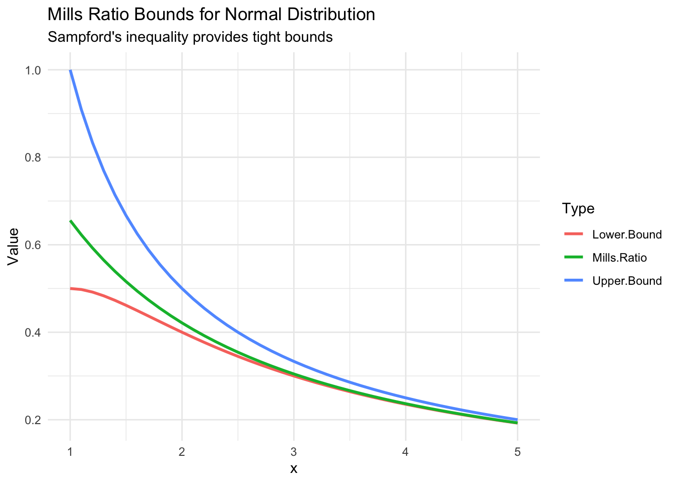

Relationship to Other Functions

Hazard Function

The hazard function (failure rate) is the reciprocal of the Mills ratio:

$h(x) = \frac{1}{m(x)} = \frac{f(x)}{\bar{F}(x)}$

Error Function

For the normal distribution:

$m(x) = \frac{\sqrt{\pi/2} \cdot \text{erfc}(x/\sqrt{2})}{\exp(-x^2/2)}$

where $\text{erfc}$ is the complementary error function.

Tail Classification

Mills ratio behavior classifies tail thickness:

Behavior	Tail Type	Example
Decreasing ( $m'(x) < 0$ )	Thin	Normal
Constant ( $m'(x) = 0$ )	Exponential	Exponential
Increasing ( $m'(x) > 0$ )	Fat	Student’s t

Applications in Statistics

Truncated Distributions

The mean of a truncated normal distribution above point $a$ is:

$E[X | X > a] = \mu + \sigma \cdot \frac{1}{m((a-\mu)/\sigma)}$

Extreme Value Theory

Mills ratios appear in the study of: - Order statistics - Record values - Peaks over threshold models

Computational Considerations

Numerical Stability

For large $x$ , direct computation can be unstable. Use:

Show code

# Unstable for large x
unstable_mills <- function(x) {
  pnorm(x, lower.tail = FALSE) / dnorm(x)
}

# Stable using log scale
stable_mills <- function(x) {
  exp(pnorm(x, lower.tail = FALSE, log.p = TRUE) - dnorm(x, log = TRUE))
}

# Compare at x = 10
x_test <- 10
c(unstable = unstable_mills(x_test),
  stable = stable_mills(x_test),
  package = mills_ratio_normal(x_test))

 unstable    stable   package
0.0990286 0.0990286 0.0990286

References

Mills, John P. 1926. “Table of the Ratio: Area to Bounding Ordinate, for Any Portion of Normal Curve.” Biometrika 18 (3/4): 395–400. https://doi.org/10.2307/2331957.

Sampford, M. R. 1953. “Some Inequalities on Mill’s Ratio and Related Functions.” The Annals of Mathematical Statistics 24 (1): 130–32. https://doi.org/10.1214/aoms/1177729093.