Overview
Mills ratios appear in diverse fields from financial risk management to reliability engineering. This article explores practical applications with working examples.
Financial Applications
Value at Risk (VaR) and Expected Shortfall
In risk management, the Mills ratio helps calculate expected losses beyond VaR:
Show code
# Portfolio with normal returns
mu <- 0.001  # Daily return
sigma <- 0.02  # Daily volatility
confidence <- 0.99  # 99% VaR

# VaR threshold (standardized)
z_var <- qnorm(1 - confidence)

# Expected shortfall using Mills ratio
mills <- mills_ratio_normal(-z_var)
expected_shortfall <- mu - sigma / mills

cat("99% VaR:", round(mu + sigma * z_var, 4), "\n")
Show code
cat("Expected Shortfall:", round(expected_shortfall, 4), "\n")
Expected Shortfall: -0.0523
Show code
cat("ES/VaR ratio:", round(expected_shortfall / (mu + sigma * z_var), 2))
Option Pricing
Mills ratios appear in exotic option formulas:
Show code
# Digital option delta using Mills ratio
digital_delta <- function(S, K, r, sigma, T) {
  d2 <- (log(S/K) + (r - 0.5*sigma^2)*T) / (sigma*sqrt(T))

  # Delta involves Mills ratio
  mills <- mills_ratio_normal(-d2)
  delta <- exp(-r*T) / (sigma * sqrt(T) * mills)

  return(delta)
}

# Example
S <- 100    # Current price
K <- 105    # Strike
r <- 0.05   # Risk-free rate
sigma <- 0.2  # Volatility
T <- 0.25   # Time to maturity

digital_delta(S, K, r, sigma, T)
Reliability Engineering
Mean Residual Life
For components with lifetime distribution, the mean residual life at age is:
Show code
# Mean residual life function
mean_residual_life <- function(t, distribution = "normal", ...) {
  if (distribution == "normal") {
    # For normal with mean mu, sd sigma
    mills <- mills_ratio_normal(t, ...)
    return(mills)
  } else if (distribution == "exponential") {
    # Constant for exponential (memoryless)
    return(mills_ratio_exp(t, ...))
  }
}

# Compare distributions
t_vals <- seq(0, 3, by = 0.5)
mrl_normal <- sapply(t_vals, mean_residual_life, distribution = "normal")
mrl_exp <- sapply(t_vals, mean_residual_life, distribution = "exponential")

data.frame(
  age = t_vals,
  normal = round(mrl_normal, 3),
  exponential = round(mrl_exp, 3)
)
  age normal exponential
1 0.0  1.253           1
2 0.5  0.876           1
3 1.0  0.656           1
4 1.5  0.516           1
5 2.0  0.421           1
6 2.5  0.354           1
7 3.0  0.305           1
System Reliability
For series systems with component lifetimes:
Show code
# Series system with n components
series_system_mills <- function(x, n_components, dist = "normal") {
  # Individual component Mills ratio
  m_component <- mills_ratio_normal(x)

  # System Mills ratio (approximation for large x)
  m_system <- m_component / n_components

  # System hazard rate
  h_system <- 1 / m_system

  return(list(
    mills_ratio = m_system,
    hazard_rate = h_system,
    mean_life = m_system
  ))
}

# 5-component system
series_system_mills(x = 2, n_components = 5)
$mills_ratio
[1] 0.08427385

$hazard_rate
[1] 11.86608

$mean_life
[1] 0.08427385
Statistical Inference
Truncated Regression
In Tobit models and truncated regression:
Show code
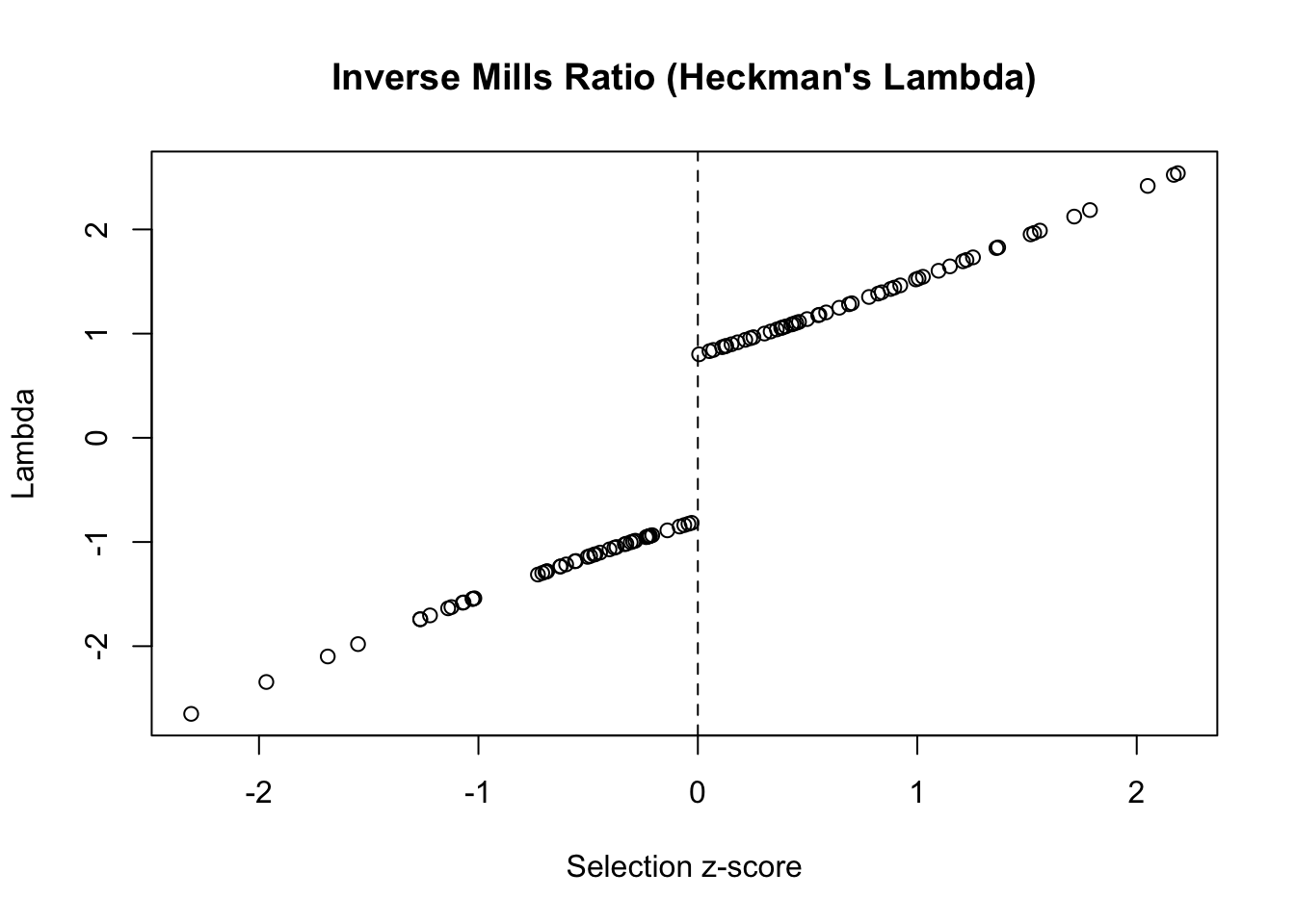
# Heckman correction using Mills ratio
heckman_correction <- function(z_scores) {
  # Selection equation produces z-scores
  selected <- z_scores > 0

  # Inverse Mills ratio for correction
  lambda <- numeric(length(z_scores))
  lambda[selected] <- 1 / mills_ratio_normal(z_scores[selected])
  lambda[!selected] <- -1 / mills_ratio_normal(-z_scores[!selected])

  return(lambda)
}

# Example with simulated data
set.seed(123)
z <- rnorm(100)
lambda <- heckman_correction(z)

plot(z, lambda,
     main = "Inverse Mills Ratio (Heckman's Lambda)",
     xlab = "Selection z-score",
     ylab = "Lambda")
abline(v = 0, lty = 2)
Survival Analysis
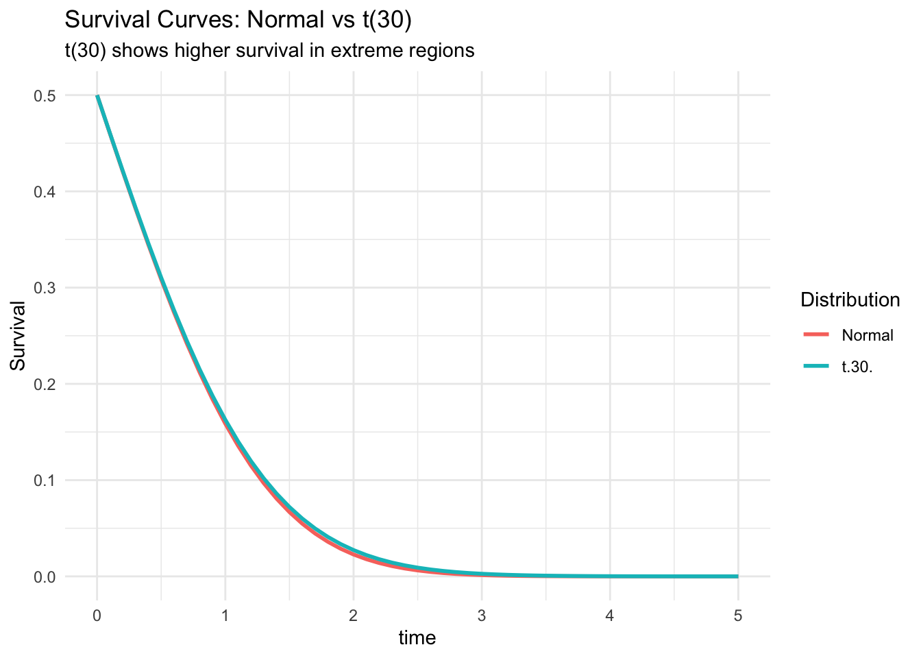
Mills ratio in survival probability calculations:
Show code
# Survival function using Mills ratio
survival_probability <- function(t, dist = "normal", ...) {
  if (dist == "normal") {
    mills <- mills_ratio_normal(t, ...)
    # S(t) = mills * f(t)
    return(mills * dnorm(t, ...))
  }
}

# Compare survival curves
t_grid <- seq(0, 5, by = 0.1)
surv_normal <- sapply(t_grid, survival_probability, dist = "normal")
surv_t30 <- pt(t_grid, df = 30, lower.tail = FALSE)

plot_data <- data.frame(
  time = t_grid,
  Normal = surv_normal,
  `t(30)` = surv_t30
) %>%
  pivot_longer(-time, names_to = "Distribution", values_to = "Survival")

ggplot(plot_data, aes(time, Survival, color = Distribution)) +
  geom_line(size = 1) +
  labs(
    title = "Survival Curves: Normal vs t(30)",
    subtitle = "t(30) shows higher survival in extreme regions"
  ) +
  theme_minimal()
Warning: Using `size` aesthetic for lines was deprecated in ggplot2 3.4.0.
ℹ Please use `linewidth` instead.
Quality Control
Process Capability
Mills ratio in capability indices:
Show code
# Enhanced process capability using Mills ratio
process_capability_mills <- function(USL, LSL, mu, sigma) {
  # Standard capability indices
  Cp <- (USL - LSL) / (6 * sigma)
  Cpk <- min((USL - mu) / (3*sigma), (mu - LSL) / (3*sigma))

  # Expected loss using Mills ratio
  z_usl <- (USL - mu) / sigma
  z_lsl <- (LSL - mu) / sigma

  mills_upper <- mills_ratio_normal(z_usl)
  mills_lower <- mills_ratio_normal(-z_lsl)

  # Expected defects per million
  dpm_upper <- 1e6 * exp(-z_usl^2/2) / (sqrt(2*pi) * mills_upper)
  dpm_lower <- 1e6 * exp(-z_lsl^2/2) / (sqrt(2*pi) * mills_lower)

  return(list(
    Cp = round(Cp, 3),
    Cpk = round(Cpk, 3),
    DPM_upper = round(dpm_upper, 1),
    DPM_lower = round(dpm_lower, 1),
    Total_DPM = round(dpm_upper + dpm_lower, 1)
  ))
}

# Six Sigma process
process_capability_mills(USL = 6, LSL = -6, mu = 0, sigma = 1)
$Cp
[1] 2

$Cpk
[1] 2

$DPM_upper
[1] 0

$DPM_lower
[1] 0

$Total_DPM
[1] 0.1
Machine Learning
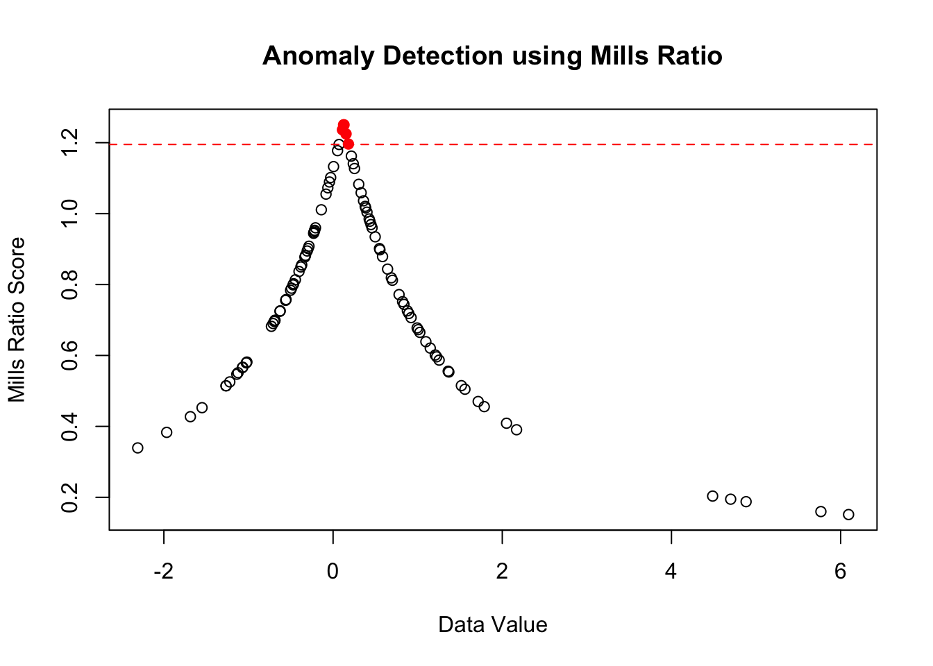
Outlier Detection
Using Mills ratio for anomaly scores:
Show code
# Anomaly score based on Mills ratio
anomaly_score <- function(x, robust = TRUE) {
  if (robust) {
    # Use median and MAD
    center <- median(x)
    scale <- mad(x)
  } else {
    center <- mean(x)
    scale <- sd(x)
  }

  # Standardize
  z <- abs(x - center) / scale

  # Mills ratio as anomaly score
  # Higher Mills ratio = more extreme
  scores <- mills_ratio_normal(z)

  return(scores)
}

# Example with contaminated data
set.seed(123)
clean_data <- rnorm(95)
outliers <- rnorm(5, mean = 5, sd = 0.5)
data <- c(clean_data, outliers)

scores <- anomaly_score(data)

# Identify outliers (high Mills ratio)
threshold <- quantile(scores, 0.95)
is_outlier <- scores > threshold

plot(data, scores,
     col = ifelse(is_outlier, "red", "black"),
     pch = ifelse(is_outlier, 19, 1),
     main = "Anomaly Detection using Mills Ratio",
     xlab = "Data Value",
     ylab = "Mills Ratio Score")
abline(h = threshold, lty = 2, col = "red")
Insurance and Actuarial Science
Excess-of-Loss Pricing
Show code
# Reinsurance premium calculation
excess_loss_premium <- function(retention, limit, mu, sigma) {
  # Standardize retention and limit
  z_ret <- (retention - mu) / sigma
  z_lim <- (retention + limit - mu) / sigma

  # Use Mills ratio for tail expectations
  mills_ret <- mills_ratio_normal(z_ret)
  mills_lim <- mills_ratio_normal(z_lim)

  # Pure premium
  premium <- sigma * (1/mills_ret - 1/mills_lim)

  return(list(
    pure_premium = premium,
    loss_probability = pnorm(z_ret, lower.tail = FALSE),
    conditional_expectation = sigma / mills_ret
  ))
}

# Example: $1M excess $500k
excess_loss_premium(
  retention = 500000,
  limit = 1000000,
  mu = 100000,
  sigma = 200000
)
$pure_premium
[1] -952866

$loss_probability
[1] 0.02275013

$conditional_expectation
[1] 474643.1
Summary
Mills ratios provide elegant solutions across diverse applications:
-
Finance: Tail risk measurement and option pricing
-
Engineering: Reliability analysis and lifetime prediction
-
Statistics: Censored data and selection bias correction
-
Quality: Process capability and defect prediction
-
ML: Anomaly detection and robust estimation
-
Insurance: Premium calculation for extreme events
The unifying theme is the characterization of tail behavior, making Mills ratios essential for any analysis involving extreme values or rare events.