Online documentation
This vignette displays pre-computed results. Run the targets pipeline locally for interactive analysis.
Overview
See the Glossary for term definitions used throughout this project.
- Compares tumor vs normal or baseline vs relapse samples
- Three complementary methods: DESeq2, edgeR, limma-voom
- Consensus genes (significant in all three) used for pathway analysis
- Visualizations: PCA, volcano plot, MA plot, heatmap, method comparison
Note: This vignette was built in CI with sample_limit=20. Local builds default to 200 samples. Numbers below reflect the CI subset.
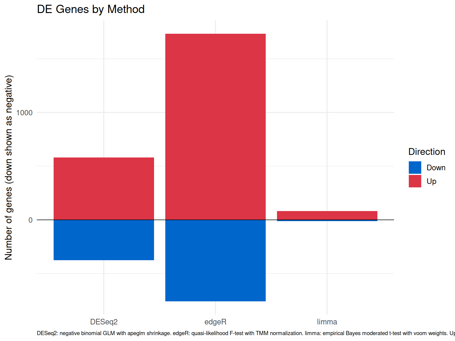
Method Comparison
Summary of DE genes detected by each method (DESeq2, edgeR, limma-voom) and their consensus overlap.
Generating code
{
    if (is.null(de_method_summary) || nrow(de_method_summary) ==
        0)
        return(NULL)
    caption <- paste0("Differential expression results across methods. ",
        "Method = DE analysis package. ", "DESeq2: negative binomial GLM with Wald test and apeglm LFC shrinkage. ",
        "edgeR: quasi-likelihood F-test with TMM normalization. ",
        "limma-voom: linear models with precision weights on log2-CPM. ",
        "Genes Tested = number of genes after filtering. ", "Significant = genes with |log2FC| > 1 AND adjusted p-value < 0.05. ",
        "Up/Down = direction of fold change (tumor vs normal).")
    DT::datatable(de_method_summary, rownames = FALSE, filter = "top",
        options = list(pageLength = 10, scrollX = TRUE), colnames = c("Method",
            "Genes Tested", "Significant", "Up", "Down"), caption = htmltools::tags$caption(style = "caption-side: top; text-align: left;",
            caption))
}
Differential expression results across methods. Method = DE analysis package. DESeq2: negative binomial GLM with Wald test and apeglm LFC shrinkage. edgeR: quasi-likelihood F-test with TMM normalization. limma-voom: linear models with precision weights on log2-CPM. Genes Tested = number of genes after filtering. Significant = genes with |log2FC| > 1 AND adjusted p-value < 0.05. Up/Down = direction of fold change (tumor vs normal).
|
method
|
n_tested
|
n_sig
|
n_up
|
n_down
|
|
DESeq2
|
30675
|
1615
|
581
|
377
|
|
edgeR
|
30675
|
3738
|
1733
|
758
|
|
limma
|
30675
|
159
|
82
|
13
|
Generating code
{
    if (is.null(de_method_summary) || nrow(de_method_summary) ==
        0)
        return(NULL)
    long <- rbind(data.frame(method = de_method_summary$method,
        direction = "Up", count = de_method_summary$n_up), data.frame(method = de_method_summary$method,
        direction = "Down", count = -de_method_summary$n_down))
    ggplot2::ggplot(long, ggplot2::aes(x = method, y = count,
        fill = direction)) + ggplot2::geom_col() + ggplot2::scale_fill_manual(values = c(Up = "#DC3545",
        Down = "#0066CC"), name = "Direction") + ggplot2::geom_hline(yintercept = 0,
        linewidth = 0.3) + ggplot2::labs(title = "DE Genes by Method",
        x = NULL, y = "Number of genes (down shown as negative)",
        caption = paste0("DESeq2: negative binomial GLM with apeglm shrinkage. ",
            "edgeR: quasi-likelihood F-test with TMM normalization. ",
            "limma: empirical Bayes moderated t-test with voom weights. ",
            "Up (red) = log2FC > 1. Down (blue) = log2FC < -1. ",
            "Thresholds: |log2FC| > 1, padj < 0.05. ", "With sample_limit=20, zero significant genes is expected. ",
            "Source: DESeq2/edgeR/limma results. ", "See method table for exact counts and annotated DE table for top genes.")) +
        ggplot2::theme_minimal(base_size = 12) + ggplot2::theme(plot.caption = ggplot2::element_text(size = 7,
        hjust = 0, lineheight = 1.2))
}
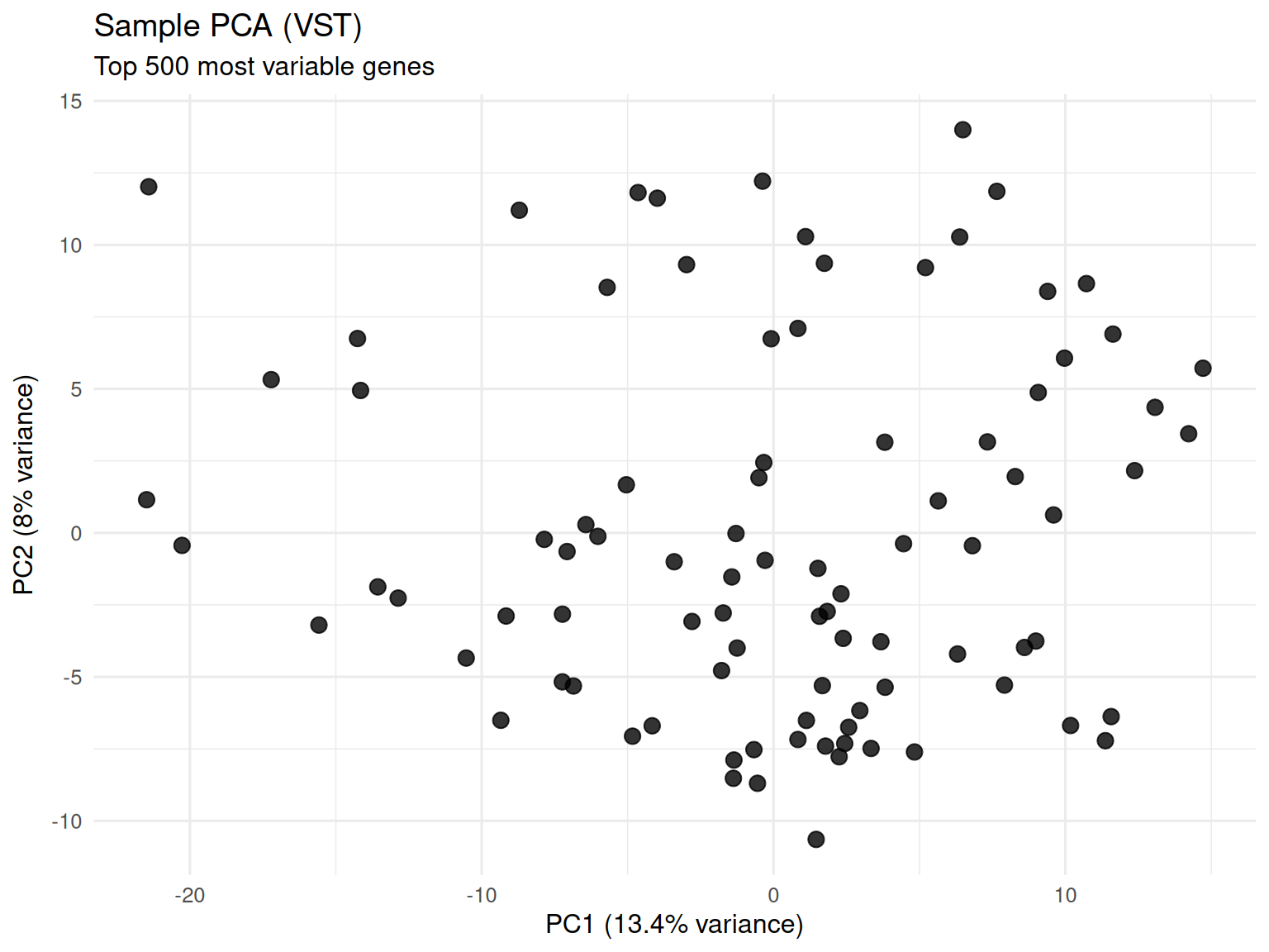
Principal Component Analysis
- Computed from top 500 most variable genes after VST
- VST stabilizes variance across the expression range
- Preferred over raw counts or logCPM for exploratory visualization
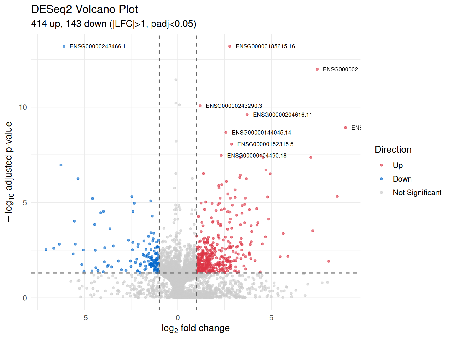
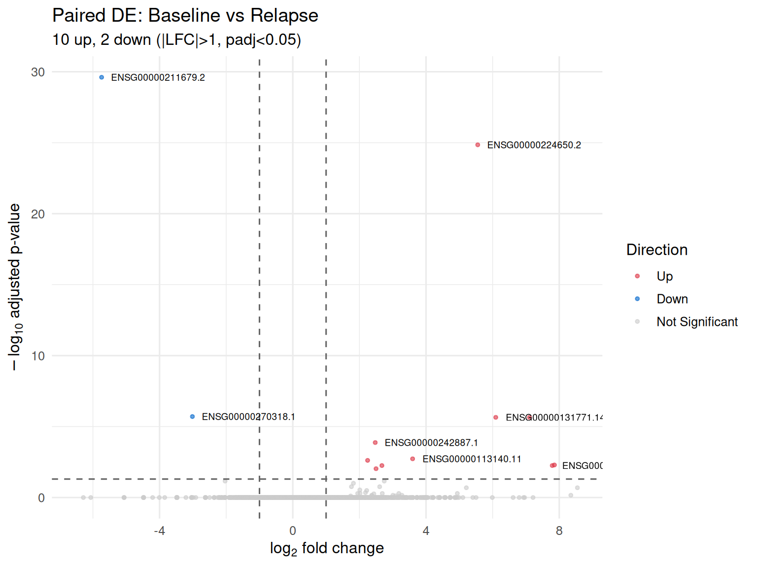
Volcano Plot
- Statistical significance (-log10 adjusted p-value) vs biological effect size (log2 fold change)
- Genes in upper corners are both statistically significant and biologically meaningful
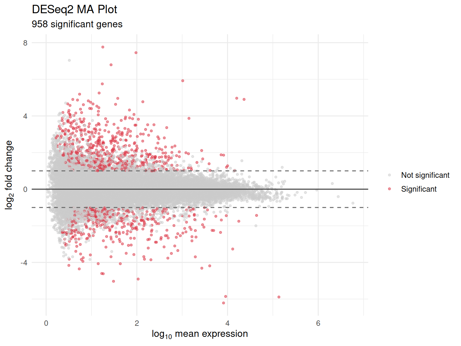
MA Plot
- Bland-Altman plot: mean expression (x-axis) vs fold change (y-axis)
- Reveals whether DE signals concentrate at particular expression levels
- Detects bias in fold-change estimates
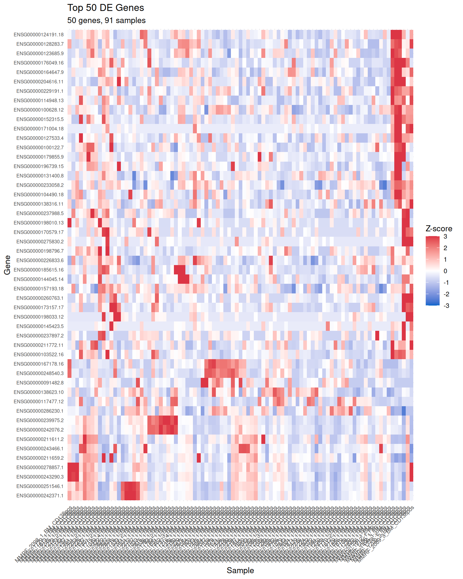
Heatmap of Top DE Genes
The heatmap shows Z-score scaled VST expression for the most significant genes. Rows (genes) and columns (samples) are hierarchically clustered.
Consensus Genes
Genes identified as significant by all three methods (DESeq2, edgeR, limma) represent the highest-confidence DE candidates.
60 consensus DE genes found across all three methods.
Top 20 consensus genes (sorted by mean rank): ENSG00000006704.11, ENSG00000027869.12, ENSG00000100065.15, ENSG00000100628.12, ENSG00000104833.12, ENSG00000106025.9, ENSG00000114948.13, ENSG00000127533.4, ENSG00000128283.7, ENSG00000130055.14, ENSG00000131711.15, ENSG00000134533.6, ENSG00000136960.13, ENSG00000138172.11, ENSG00000143341.12, ENSG00000149742.10, ENSG00000154734.16, ENSG00000157214.14, ENSG00000162878.13, ENSG00000163362.11, … (40 more)
These genes are used for pathway analysis via ORA.
Paired Longitudinal DE
For patients with samples at multiple timepoints (baseline and relapse), a paired design (~ patient_id + visit) controls for inter-patient variability and tests for within-patient expression changes over time.
Paired analysis: 2 patients, 4 samples
12 DE genes at padj < 0.05
Annotated DE Results
Gene symbols make Ensembl IDs interpretable. The annotate_genes() function maps Ensembl IDs to HGNC symbols using MSigDB gene mappings.
Generating code
{
    if (is.null(de_results_annotated) || nrow(de_results_annotated) ==
        0) {
        return(NULL)
    }
    top <- utils::head(de_results_annotated[order(de_results_annotated$padj),
        ], 15)
    display_cols <- intersect(c("gene_symbol", "log2FoldChange",
        "baseMean", "padj"), names(top))
    if ("log2FoldChange" %in% names(top))
        top$log2FoldChange <- round(top$log2FoldChange, 2)
    if ("baseMean" %in% names(top))
        top$baseMean <- round(top$baseMean, 1)
    if ("padj" %in% names(top))
        top$padj <- signif(top$padj, 4)
    caption <- paste0("Top 15 DE genes by adjusted p-value (DESeq2). ",
        "gene_symbol = HGNC symbol mapped from Ensembl IDs via MSigDB. ",
        "log2FoldChange = log2 ratio (positive = upregulated in tumor/relapse). ",
        "baseMean = mean normalized count across all samples. ",
        "padj = Benjamini-Hochberg adjusted p-value. ", "See data dictionary for gene ID details.")
    DT::datatable(top[, display_cols], rownames = FALSE, filter = "top",
        options = list(pageLength = 15, scrollX = TRUE), caption = htmltools::tags$caption(style = "caption-side: top; text-align: left;",
            caption))
}
Top 15 DE genes by adjusted p-value (DESeq2). gene_symbol = HGNC symbol mapped from Ensembl IDs via MSigDB. log2FoldChange = log2 ratio (positive = upregulated in tumor/relapse). baseMean = mean normalized count across all samples. padj = Benjamini-Hochberg adjusted p-value. See data dictionary for gene ID details.
|
gene_symbol
|
log2FoldChange
|
baseMean
|
padj
|
|
PDIA2
|
2.78
|
1027.4
|
0
|
|
IGKV1-5
|
-6.09
|
135865.3
|
0
|
|
IGLV3-25
|
7.46
|
23154.4
|
0
|
|
IGKV1-33
|
-0.10
|
8165.9
|
0
|
|
IGKV1D-33
|
-0.10
|
9086.9
|
0
|
|
GIPC3
|
0.09
|
33.0
|
0
|
|
IGKV1-12
|
1.20
|
15950.1
|
0
|
|
TRIM31
|
3.71
|
54.4
|
0
|
|
HS6ST2
|
8.98
|
16.8
|
0
|
|
DQX1
|
2.58
|
55.9
|
0
|
|
LOC283731
|
-0.09
|
106.0
|
0
|
|
KCNK13
|
2.88
|
85.5
|
0
|
|
NCALD
|
2.32
|
207.8
|
0
|
|
ADAM23
|
4.45
|
46.7
|
0
|
|
STEAP1
|
3.34
|
90.2
|
0
|
Pathway Enrichment Visualizations
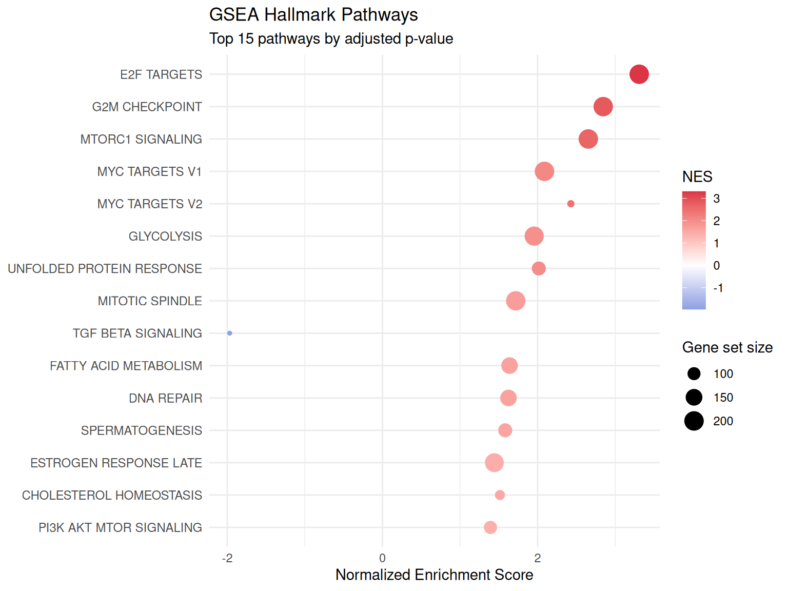
GSEA Enrichment Dot Plot
Gene Set Enrichment Analysis using the full ranked gene list against MSigDB Hallmark pathways.
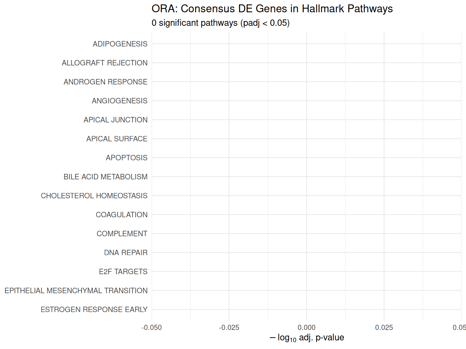
ORA Enrichment Bar Plot
Over-representation analysis testing whether consensus DE genes are enriched in specific pathways.
Next Steps
-
Pathway analysis: Consensus DE genes are tested for enrichment in MSigDB Hallmark, KEGG, and other collections. See the pathway analysis vignette.
-
Survival stratification: DE gene signatures can inform survival analysis. See the survival analysis vignette.
-
Cytogenetic context: See the EDA vignette for the cytogenetic landscape underlying these expression changes.
Data Sources
Results in this vignette are derived from the MMRF CoMMpass study (MMRF-COMMPASS, ~1,143 patients), downloaded via TCGAbiolinks. The pipeline runs with a configurable sample_limit (default 200; CI uses 20).
For full citations, data access tiers, and the distinction between pipeline data and synthetic test data, see the Data Sources vignette.
Recent Changes
Recent project commits with lines added, files changed, and change categories.
Last 20 project commits with change statistics. Date = commit date; Type = conventional-commit prefix (feat/fix/docs/ci/refactor/test/chore). Files = number of files modified; +Lines/-Lines = lines added/removed. Source: git log –numstat. See changes-by-type table for aggregate breakdown.
|
date
|
type
|
summary
|
n_files
|
lines_added
|
lines_removed
|
file_categories
|
|
2026-03-14
|
Bug Fix
|
fix(pipeline): Fix 11 NULL targets — DE condition, ID matching, consensus type
|
41
|
146
|
47
|
Other, R Source
|
|
2026-03-14
|
Bug Fix
|
fix(cachix): Remove –watch-mode auto flag (already default)
|
1
|
1
|
1
|
Other
|
|
2026-03-14
|
Bug Fix
|
fix(pipeline): Fix 3 NULL-target bugs, auto-generate package.nix (#93)
|
87
|
235
|
80
|
Config, Docs, Other, R Source
|
|
2026-03-14
|
Bug Fix
|
fix(nix): Fix cachix signing key, rebuild Bioconductor-dependent targets
|
2
|
0
|
0
|
Other
|
|
2026-03-14
|
New Feature
|
feat(captions): Add dynamic captions to 34 table/plot targets
|
22
|
579
|
89
|
Other, R Source
|
|
2026-03-14
|
Bug Fix
|
fix(vignettes): Enforce zero-computation rule — 22 violations → 0
|
32
|
360
|
764
|
Other, R Source, Vignettes
|
|
2026-03-13
|
Bug Fix
|
fix(vignettes): Convert kable RDS to data.frames, fix telemetry eval guards
|
18
|
8
|
2
|
Other, Vignettes
|
|
2026-03-13
|
Bug Fix
|
fix(ci): Save data frames (not DT widgets) to RDS for Nix portability
|
3
|
0
|
0
|
Other
|
|
2026-03-13
|
Bug Fix
|
fix(vignettes): Use Quarto #| eval syntax for pkgdown-banner chunks
|
11
|
44
|
11
|
Vignettes
|
|
2026-03-13
|
Refactoring
|
refactor(targets): Move Bioconductor packages to per-target declarations
|
11
|
35
|
17
|
Other, R Source, Vignettes
|
|
2026-03-13
|
New Feature
|
feat(vignettes): Add code provenance, kable→DT conversion, caption compliance
|
35
|
1004
|
437
|
CI/CD, Other, R Source, Vignettes
|
|
2026-03-13
|
Bug Fix
|
fix(vignettes): Skip NULL RDS in safe_tar_read, return invisible(NULL)
|
11
|
22
|
22
|
Vignettes
|
|
2026-03-13
|
Bug Fix
|
fix(glossary): Prevent double DT::datatable() wrapping in glossary-table chunk
|
1
|
3
|
1
|
Vignettes
|
|
2026-03-13
|
CI/CD
|
ci: Show quarto errors with quiet=FALSE, render individual vignettes in diagnostic
|
1
|
20
|
6
|
CI/CD
|
|
2026-03-13
|
CI/CD
|
ci: Add verbose quarto error diagnostics on build failure
|
1
|
14
|
1
|
CI/CD
|
|
2026-03-13
|
Bug Fix
|
fix(vignettes): Strip Nix paths from DT widgets, auto-wrap data frames
|
25
|
66
|
28
|
CI/CD, Other, Vignettes
|
|
2026-03-13
|
CI/CD
|
ci: Add diagnostic quarto render step to debug build failure
|
1
|
17
|
0
|
CI/CD
|
|
2026-03-13
|
Bug Fix
|
fix(vignettes): Revert safe_tar_read placeholder, guard gene-report
|
11
|
12
|
56
|
Vignettes
|
|
2026-03-13
|
Maintenance
|
chore: Export vig_count_distribution_plot as ggplot RDS (513KB)
|
1
|
0
|
0
|
Other
|
|
2026-03-13
|
Bug Fix
|
fix(vignettes): Enable code eval in CI with RDS fallback
|
80
|
113
|
74
|
CI/CD, Other, R Source, Vignettes
|
Reproducibility
Session Info (click to expand)
Show code
sessionInfo()
#> R version 4.5.3 (2026-03-11)
#> Platform: x86_64-pc-linux-gnu
#> Running under: Ubuntu 24.04.3 LTS
#>
#> Matrix products: default
#> BLAS:   /usr/lib/x86_64-linux-gnu/openblas-pthread/libblas.so.3
#> LAPACK: /usr/lib/x86_64-linux-gnu/openblas-pthread/libopenblasp-r0.3.26.so;  LAPACK version 3.12.0
#>
#> locale:
#>  [1] LC_CTYPE=C.UTF-8       LC_NUMERIC=C           LC_TIME=C.UTF-8
#>  [4] LC_COLLATE=C.UTF-8     LC_MONETARY=C.UTF-8    LC_MESSAGES=C.UTF-8
#>  [7] LC_PAPER=C.UTF-8       LC_NAME=C              LC_ADDRESS=C
#> [10] LC_TELEPHONE=C         LC_MEASUREMENT=C.UTF-8 LC_IDENTIFICATION=C
#>
#> time zone: UTC
#> tzcode source: system (glibc)
#>
#> attached base packages:
#> [1] stats     graphics  grDevices utils     datasets  methods   base
#>
#> loaded via a namespace (and not attached):
#>  [1] base64url_1.4       gtable_0.3.6        jsonlite_2.0.0
#>  [4] dplyr_1.2.0         compiler_4.5.3      tidyselect_1.2.1
#>  [7] callr_3.7.6         scales_1.4.0        yaml_2.3.12
#> [10] fastmap_1.2.0       ggplot2_4.0.2       R6_2.6.1
#> [13] labeling_0.4.3      generics_0.1.4      igraph_2.2.2
#> [16] knitr_1.51          backports_1.5.0     targets_1.12.0
#> [19] tibble_3.3.1        pillar_1.11.1       RColorBrewer_1.1-3
#> [22] rlang_1.1.7         xfun_0.57           S7_0.2.1
#> [25] otel_0.2.0          cli_3.6.5           withr_3.0.2
#> [28] magrittr_2.0.4      ps_1.9.1            digest_0.6.39
#> [31] grid_4.5.3          processx_3.8.6      secretbase_1.2.0
#> [34] lifecycle_1.0.5     prettyunits_1.2.0   vctrs_0.7.2
#> [37] evaluate_1.0.5      glue_1.8.0          data.table_1.18.2.1
#> [40] farver_2.1.2        codetools_0.2-20    rmarkdown_2.30
#> [43] tools_4.5.3         pkgconfig_2.0.3     htmltools_0.5.9