Telemetry, Coverage, and Pipeline Performance

Pipeline metrics, code coverage, memory usage, and targets dependency visualization

Author

randomwalk package

Published

January 1, 2026

Overview

This vignette presents comprehensive telemetry for the randomwalk package:

Code Coverage: Test coverage analysis using covr
Pipeline Performance: Execution time and memory usage via targets
Network Visualization: Pipeline dependency graph
Performance Hotspots: Longest-running targets and memory hogs
System Information: Environment and reproducibility details

All metrics are pre-computed using the targets pipeline and loaded via tar_read().

Package Information

Show code

# Load package metadata from targets pipeline
pkg_info <- tar_read(package_info)

# Display as formatted table
data.frame(
  Field = c("Package", "Version", "Title", "Generated"),
  Value = c(
    pkg_info$package,
    pkg_info$version,
    pkg_info$title,
    format(pkg_info$date, "%Y-%m-%d")
  )
) %>%
  kable(caption = "Package Metadata")

Package Metadata
	Field	Value
Package	Package	randomwalk
Version	Version	2.1.0
Title	Title	Asynchronous Pixel Walking Simulation with Parallel Processing
	Generated	2025-12-28

Code Coverage Analysis

Test coverage provides insight into which code paths are exercised by the test suite.

Overall Coverage

Show code

# Load pre-computed coverage from targets pipeline (if available)
cov_data <- tryCatch({
  tar_read(code_coverage)
}, error = function(e) NULL)

cov_available <- !is.null(cov_data)

if (cov_available) {
  cat(sprintf("Overall Test Coverage: %.1f%%\n", cov_data$overall_pct))
} else {
  cat("⚠️ Code coverage analysis is temporarily disabled.\n\n")
  cat("The covr::package_coverage() function encounters 'error reading from connection'\n")
  cat("in Nix environments. This is a known compatibility issue being tracked.\n\n")
  cat("To generate coverage locally:\n")
  cat("  coverage <- covr::package_coverage()\n")
  cat("  covr::report(coverage)\n")
}

⚠️ Code coverage analysis is temporarily disabled.

The covr::package_coverage() function encounters 'error reading from connection'
in Nix environments. This is a known compatibility issue being tracked.

To generate coverage locally:
  coverage <- covr::package_coverage()
  covr::report(coverage)

Coverage by File

Show code

# Use pre-computed file summary from targets (if available)
if (cov_available) {
  file_summary <- cov_data$file_summary

  file_summary %>%
    kable(
      digits = 1,
      col.names = c("File", "Total Lines", "Covered Lines", "Coverage (%)"),
      caption = "Test Coverage by File"
    )
} else {
  cat("Coverage data not available - code_coverage target is disabled\n")
}

Coverage data not available - code_coverage target is disabled

Coverage Visualization

Show code

if (cov_available) {
  file_summary %>%
    mutate(filename = reorder(filename, coverage_pct)) %>%
    ggplot(aes(x = filename, y = coverage_pct)) +
    geom_col(aes(fill = coverage_pct), alpha = 0.8) +
    geom_hline(yintercept = 80, linetype = "dashed", color = "red") +
    scale_fill_gradient2(
      low = "red", mid = "yellow", high = "green",
      midpoint = 50, limits = c(0, 100),
      name = "Coverage %"
    ) +
    coord_flip() +
    labs(
      title = "Test Coverage by File",
      subtitle = "Dashed line shows 80% coverage target",
      x = "File",
      y = "Coverage (%)"
    ) +
    theme_minimal() +
    theme(legend.position = "bottom")
} else {
  cat("Coverage visualization not available - code_coverage target is disabled\n")
}

Coverage visualization not available - code_coverage target is disabled

Untested Code Hotspots

Files with low coverage that need additional tests:

Show code

if (cov_available) {
  low_coverage <- file_summary %>%
    filter(coverage_pct < 80) %>%
    arrange(coverage_pct)

  if (nrow(low_coverage) > 0) {
    low_coverage %>%
      kable(
        digits = 1,
        col.names = c("File", "Total Lines", "Covered Lines", "Coverage (%)"),
        caption = "Files Below 80% Coverage (Need More Tests)"
      )
  } else {
    cat("✅ All files have >80% coverage!\n")
  }
} else {
  cat("Coverage data not available - code_coverage target is disabled\n")
}

Coverage data not available - code_coverage target is disabled

Pipeline Performance Telemetry

Pipeline Network Visualization

The targets pipeline dependency graph shows how targets depend on each other:

Show code

# Visualize the pipeline network
tar_visnetwork(
  targets_only = TRUE,
  label = c("time", "size", "branches")
)

Interactive: Click and drag nodes to explore dependencies. Hover for details.

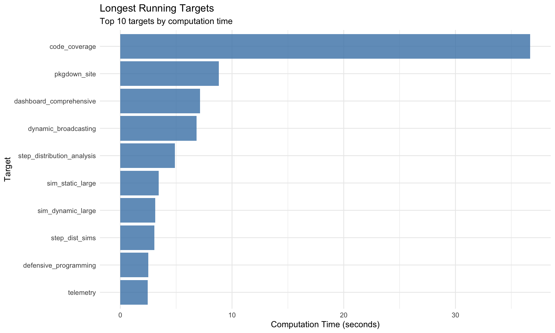
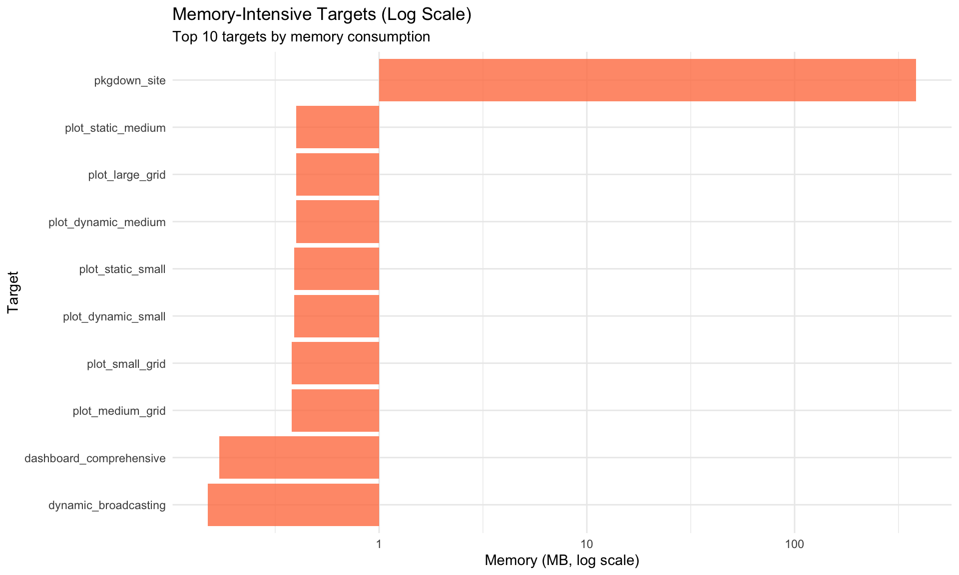
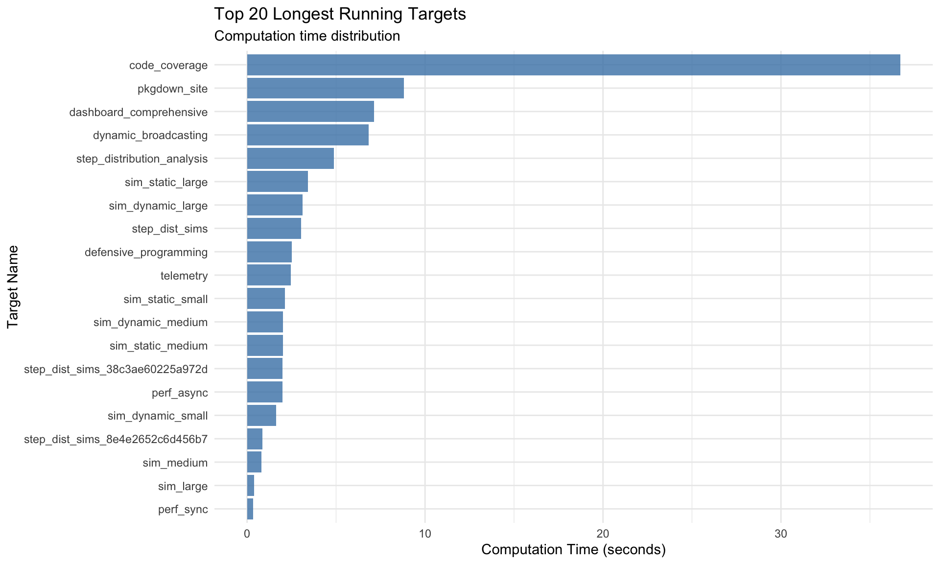
Target Execution Statistics

Summary Table

Show code

# Generate telemetry from tar_meta() - safe to call AFTER pipeline completes
telemetry <- tar_meta() %>%
  mutate(
    time_seconds = as.numeric(seconds, units = "secs"),
    time_formatted = sprintf("%.2fs", time_seconds),
    memory_mb = round(bytes / 1024^2, 2),
    status = ifelse(is.na(error), "✅ success", "❌ error")
  ) %>%
  filter(!is.na(time_seconds))

# Display sortable/filterable table using DT
telemetry %>%
  select(name, time_seconds, memory_mb, status) %>%
  rename(
    "Target Name" = name,
    "Time (sec)" = time_seconds,
    "Memory (MB)" = memory_mb,
    "Status" = status
  ) %>%
  datatable(
    caption = "Target Pipeline Execution Summary (click columns to sort, use search to filter)",
    filter = "top",
    options = list(
      pageLength = 15,
      order = list(list(1, "desc")),  # Sort by time descending
      columnDefs = list(
        list(className = "dt-right", targets = c(1, 2))
      )
    ),
    rownames = FALSE
  ) %>%
  formatRound(columns = c("Time (sec)", "Memory (MB)"), digits = 2)

Performance Metrics

Show code

# Calculate summary statistics
total_time <- sum(telemetry$time_seconds, na.rm = TRUE)
total_memory <- sum(telemetry$memory_mb, na.rm = TRUE)
target_count <- nrow(telemetry)

data.frame(
  Metric = c("Total Targets", "Total Computation Time", "Total Memory Usage", "Average Time/Target", "Average Memory/Target"),
  Value = c(
    target_count,
    sprintf("%.1f seconds", total_time),
    sprintf("%.1f MB", total_memory),
    sprintf("%.2f seconds", total_time / target_count),
    sprintf("%.2f MB", total_memory / target_count)
  )
) %>%
  kable(caption = "Pipeline Performance Summary")

Pipeline Performance Summary
Metric	Value
Total Targets	38
Total Computation Time	94.1 seconds
Total Memory Usage	389.2 MB
Average Time/Target	2.48 seconds
Average Memory/Target	10.24 MB

Longest Running Targets

Targets that take the most time to compute:

Show code

# Top 10 longest running targets
longest <- telemetry %>%
  arrange(desc(time_seconds)) %>%
  head(10) %>%
  select(name, time_formatted, memory_mb)

longest %>%
  kable(
    col.names = c("Target", "Computation Time", "Memory (MB)"),
    caption = "Top 10 Longest Running Targets"
  )

Top 10 Longest Running Targets
Target	Computation Time	Memory (MB)
code_coverage	36.70s	0.00
pkgdown_site	8.81s	385.19
dashboard_comprehensive	7.15s	0.17
dynamic_broadcasting	6.82s	0.15
step_distribution_analysis	4.88s	0.13
sim_static_large	3.42s	0.12
sim_dynamic_large	3.11s	0.13
step_dist_sims	3.04s	0.10
defensive_programming	2.52s	0.13
telemetry	2.46s	0.13

Longest Running Targets Visualization

Show code

longest %>%
  mutate(
    name = reorder(name, telemetry$time_seconds[match(name, telemetry$name)]),
    time_secs = telemetry$time_seconds[match(name, telemetry$name)]
  ) %>%
  ggplot(aes(x = name, y = time_secs)) +
  geom_col(fill = "steelblue", alpha = 0.8) +
  coord_flip() +
  labs(
    title = "Longest Running Targets",
    subtitle = "Top 10 targets by computation time",
    x = "Target",
    y = "Computation Time (seconds)"
  ) +
  theme_minimal()

Optimization Opportunities: Consider caching or optimizing these targets to improve pipeline performance.

Highest Memory Targets

Targets that consume the most memory:

Show code

# Top 10 highest memory targets
memory_hogs <- telemetry %>%
  arrange(desc(memory_mb)) %>%
  head(10) %>%
  select(name, memory_mb, time_formatted)

memory_hogs %>%
  kable(
    col.names = c("Target", "Memory (MB)", "Computation Time"),
    caption = "Top 10 Memory-Intensive Targets"
  )

Top 10 Memory-Intensive Targets
Target	Memory (MB)	Computation Time
pkgdown_site	385.19	8.81s
plot_large_grid	0.40	0.09s
plot_static_medium	0.40	0.09s
plot_dynamic_medium	0.40	0.09s
plot_static_small	0.39	0.11s
plot_dynamic_small	0.39	0.09s
plot_medium_grid	0.38	0.09s
plot_small_grid	0.38	0.09s
dashboard_comprehensive	0.17	7.15s
dynamic_broadcasting	0.15	6.82s

Memory Usage Visualization

Show code

memory_hogs %>%
  mutate(
    name = reorder(name, telemetry$memory_mb[match(name, telemetry$name)]),
    memory = telemetry$memory_mb[match(name, telemetry$name)]
  ) %>%
  ggplot(aes(x = name, y = memory)) +
  geom_col(fill = "coral", alpha = 0.8) +
  coord_flip() +
  scale_y_log10(labels = scales::comma_format()) +
  labs(
    title = "Memory-Intensive Targets (Log Scale)",
    subtitle = "Top 10 targets by memory consumption",
    x = "Target",
    y = "Memory (MB, log scale)"
  ) +
  theme_minimal()

Top 10 memory-intensive targets (log scale)

Storage Optimization: High-memory targets may benefit from compression or data format optimization.

Computation Time Distribution

Show code

telemetry %>%
  arrange(desc(time_seconds)) %>%
  head(20) %>%
  mutate(name = reorder(name, time_seconds)) %>%
  ggplot(aes(x = name, y = time_seconds)) +
  geom_col(fill = "steelblue", alpha = 0.8) +
  coord_flip() +
  labs(
    title = "Top 20 Longest Running Targets",
    subtitle = "Computation time distribution",
    x = "Target Name",
    y = "Computation Time (seconds)"
  ) +
  theme_minimal()

Computation time distribution across all targets

Memory Usage Distribution

Show code

telemetry %>%
  arrange(desc(memory_mb)) %>%
  head(20) %>%
  mutate(name = reorder(name, memory_mb)) %>%
  ggplot(aes(x = name, y = memory_mb)) +
  geom_col(fill = "coral", alpha = 0.8) +
  coord_flip() +
  scale_y_log10(labels = scales::comma_format()) +
  labs(
    title = "Top 20 Memory-Intensive Targets (Log Scale)",
    subtitle = "Memory usage distribution",
    x = "Target Name",
    y = "Memory (MB, log scale)"
  ) +
  theme_minimal()

Memory usage distribution across all targets (log scale)

Performance Trends

Time vs Memory Scatter

Relationship between computation time and memory usage (log-log scale for better visualization of range):

Show code

# Filter out zero/NA values for log scale
plot_data <- telemetry %>%
  filter(time_seconds > 0, memory_mb > 0)

plot_data %>%
  ggplot(aes(x = time_seconds, y = memory_mb)) +
  geom_point(aes(color = status), size = 3, alpha = 0.7) +
  geom_text(
    data = plot_data %>% filter(time_seconds > quantile(time_seconds, 0.9) | memory_mb > quantile(memory_mb, 0.9)),
    aes(label = name),
    hjust = -0.1,
    vjust = -0.1,
    size = 3,
    check_overlap = TRUE
  ) +
  scale_x_log10(labels = scales::comma_format()) +
  scale_y_log10(labels = scales::comma_format()) +
  scale_color_manual(
    values = c("✅ success" = "steelblue", "❌ error" = "red"),
    name = "Status"
  ) +
  labs(
    title = "Target Performance: Time vs Memory (Log-Log Scale)",
    subtitle = "Outliers labeled; log scale reveals patterns across orders of magnitude",
    x = "Computation Time (seconds, log scale)",
    y = "Memory (MB, log scale)"
  ) +
  theme_minimal() +
  theme(legend.position = "bottom")

Computation time vs memory usage (log-log scale)

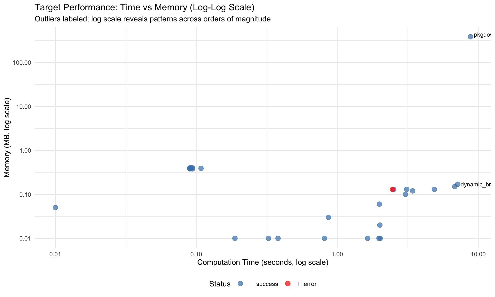
Key Observations: - Targets in upper-right quadrant (high time, high memory) are optimization candidates - Targets with disproportionate time/memory ratios may have inefficiencies

Example Simulations

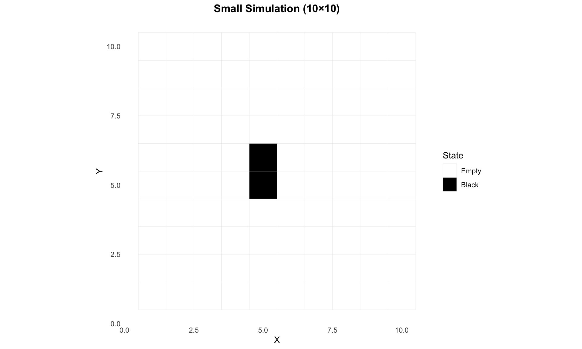
Small Simulation

A small 10×10 grid simulation with 3 walkers:

Show code

# Load pre-computed statistics
stats_small <- tar_read(stats_small)

# Display statistics
if (is.data.frame(stats_small) || is.list(stats_small)) {
  print(stats_small)
} else {
  cat("Statistics available but format not suitable for display\n")
}

$black_pixels
[1] 2

$black_percentage
[1] 2

$grid_size
[1] 10

$total_walkers
[1] 3

$completed_walkers
[1] 3

$total_steps
[1] 7

$min_steps
[1] 0

$max_steps
[1] 6

$mean_steps
[1] 2.333333

$median_steps
[1] 1

$percentile_25
25% 
0.5 

$percentile_75
75% 
3.5 

$elapsed_time_secs
[1] 0.00956893

$termination_reasons

black_neighbor   hit_boundary 
             1              2

Show code

# Load pre-computed plot
tar_read(plot_small_grid)

Medium Simulation

A medium 20×20 grid simulation with 5 walkers:

Show code

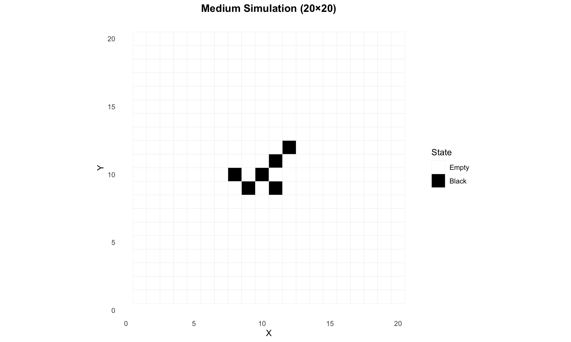
# Load pre-computed statistics
stats_medium <- tar_read(stats_medium)

# Display statistics
if (is.data.frame(stats_medium) || is.list(stats_medium)) {
  print(stats_medium)
} else {
  cat("Statistics available but format not suitable for display\n")
}

$black_pixels
[1] 6

$black_percentage
[1] 1.5

$grid_size
[1] 20

$total_walkers
[1] 5

$completed_walkers
[1] 5

$total_steps
[1] 3163

$min_steps
[1] 308

$max_steps
[1] 1205

$mean_steps
[1] 632.6

$median_steps
[1] 582

$percentile_25
25% 
434 

$percentile_75
75% 
634 

$elapsed_time_secs
[1] 0.230211

$termination_reasons

black_neighbor 
             5

Show code

# Load pre-computed plot
tar_read(plot_medium_grid)

System Information

R Session Information

Complete session information including R version, platform, and loaded packages:

Show code

# Load session info from targets pipeline
sess_info <- tar_read(session_info)

# Display formatted session info
print(sess_info)

R version 4.5.2 (2025-10-31)
Platform: aarch64-apple-darwin24.6.0
Running under: macOS Sequoia 15.7.1

Matrix products: default
BLAS:   /nix/store/jammm5gz621n7dkzfzc1c43gs6xv9a10-blas-3/lib/libblas.dylib 
LAPACK: /nix/store/30ypx3jnyq4r1z4nv742j1csfflsd66v-openblas-0.3.30/lib/libopenblasp-r0.3.30.dylib;  LAPACK version 3.12.0

locale:
[1] en_US.UTF-8/en_US.UTF-8/en_US.UTF-8/C/en_US.UTF-8/en_US.UTF-8

time zone: UTC
tzcode source: internal

attached base packages:
[1] stats     graphics  grDevices utils     datasets  methods   base     

other attached packages:
 [1] randomwalk_2.1.0   testthat_3.2.3     quarto_1.5.1       pkgdown_2.1.3     
 [5] logger_0.4.1       ggplot2_4.0.0      DT_0.34.0          dplyr_1.1.4       
 [9] devtools_2.4.6     usethis_3.2.1      tarchetypes_0.13.2 targets_1.11.4    

loaded via a namespace (and not attached):
 [1] gtable_0.3.6       xfun_0.54          htmlwidgets_1.6.4  remotes_2.5.0     
 [5] processx_3.8.6     callr_3.7.6        vctrs_0.6.5        tools_4.5.2       
 [9] ps_1.9.1           generics_0.1.4     base64url_1.4      parallel_4.5.2    
[13] tibble_3.3.0       pkgconfig_2.0.3    mirai_2.5.1        data.table_1.17.8 
[17] secretbase_1.0.5   RColorBrewer_1.1-3 S7_0.2.0           desc_1.4.3        
[21] lifecycle_1.0.4    compiler_4.5.2     farver_2.1.2       brio_1.1.5        
[25] codetools_0.2-20   htmltools_0.5.8.1  yaml_2.3.10        later_1.4.4       
[29] pillar_1.11.1      crew_1.3.0         ellipsis_0.3.2     autometric_0.1.2  
[33] cachem_1.1.0       sessioninfo_1.2.3  tidyselect_1.2.1   digest_0.6.37     
[37] purrr_1.1.0        rprojroot_2.1.1    fastmap_1.2.0      grid_4.5.2        
[41] cli_3.6.5          magrittr_2.0.4     pkgbuild_1.4.8     withr_3.0.2       
[45] promises_1.5.0     prettyunits_1.2.0  scales_1.4.0       backports_1.5.0   
[49] rmarkdown_2.30     otel_0.2.0         igraph_2.2.1       memoise_2.0.1     
[53] evaluate_1.0.5     knitr_1.50         rlang_1.1.6        Rcpp_1.1.0        
[57] nanonext_1.7.2     glue_1.8.0         collections_0.3.9  pkgload_1.4.1     
[61] rstudioapi_0.17.1  jsonlite_2.0.0     R6_2.6.1           fs_1.6.6

Git/GitHub Summary

Version control and repository information:

Show code

# Load git summary from targets pipeline
git_info <- tar_read(git_summary)

# Display as formatted table
data.frame(
  Field = c("Branch", "Commit", "Remote", "Status"),
  Value = c(
    git_info$branch,
    git_info$commit,
    basename(git_info$remote),
    if (length(git_info$status) == 0) "Clean" else "Modified"
  )
) %>%
  kable(caption = "Git Repository Information")

Git Repository Information
Field	Value
Branch	main
Commit	f6e034c
Remote	randomwalk.git
Status	Modified

Pipeline Reproducibility

All objects displayed in this vignette are pre-computed and stored in the targets pipeline. To reproduce these results:

Ensure you have the required packages installed (see DESCRIPTION)
Run targets::tar_make() to execute the pipeline
Render this vignette to see the updated results

Show code

# Reproduce the pipeline
targets::tar_make()

# View the pipeline network
targets::tar_visnetwork()

# Check target status
targets::tar_meta()

# View longest-running targets
tar_meta() %>%
  arrange(desc(seconds)) %>%
  select(name, seconds, bytes) %>%
  head(10)

# Generate coverage report
library(covr)
coverage <- package_coverage()
report(coverage)

Performance Recommendations

Based on the telemetry analysis:

High-Priority Optimizations

Show code

# Identify optimization candidates
candidates <- telemetry %>%
  mutate(
    time_percentile = percent_rank(time_seconds),
    memory_percentile = percent_rank(memory_mb),
    priority_score = time_percentile + memory_percentile
  ) %>%
  filter(priority_score > 1.5) %>%  # Top 25% in both dimensions
  arrange(desc(priority_score)) %>%
  select(name, time_formatted, memory_mb, priority_score)

if (nrow(candidates) > 0) {
  candidates %>%
    kable(
      digits = 2,
      col.names = c("Target", "Time", "Memory (MB)", "Priority Score"),
      caption = "Optimization Candidates (High Time + High Memory)"
    )
} else {
  cat("No high-priority optimization candidates identified.\n")
}

Optimization Candidates (High Time + High Memory)
Target	Time	Memory (MB)	Priority Score
pkgdown_site	8.81s	385.19	1.97
dashboard_comprehensive	7.15s	0.17	1.73
dynamic_broadcasting	6.82s	0.15	1.68
step_distribution_analysis	4.88s	0.13	1.54

Recommended Actions

Cache expensive targets: Use tar_target(format = "qs") for large objects
Parallelize independent targets: Use tar_make_future() or tar_make_clustermq()
Optimize algorithms: Review code for longest-running targets
Reduce memory footprint: Use memory-efficient data structures
Add test coverage: Focus on files with <80% coverage

Summary

This telemetry vignette provides comprehensive performance insights:

Code Coverage: covr package analysis identifies untested code
Pipeline Performance: Execution time and memory usage per target
Performance Hotspots: Longest-running and memory-intensive targets identified
Network Visualization: tar_visnetwork() shows pipeline dependencies
Optimization Guidance: Data-driven recommendations for improvements
Reproducibility: Version control and system information

All statistics are generated automatically from the targets pipeline, ensuring consistency across builds.

Generated on: 2026-01-01 15:22:42.234013

Using targets pipeline from: _targets.R

Session Info

Show code

sessionInfo()

R version 4.5.2 (2025-10-31)
Platform: aarch64-apple-darwin24.6.0
Running under: macOS Sequoia 15.7.1

Matrix products: default
BLAS:   /nix/store/jammm5gz621n7dkzfzc1c43gs6xv9a10-blas-3/lib/libblas.dylib 
LAPACK: /nix/store/30ypx3jnyq4r1z4nv742j1csfflsd66v-openblas-0.3.30/lib/libopenblasp-r0.3.30.dylib;  LAPACK version 3.12.0

locale:
[1] en_US.UTF-8/en_US.UTF-8/en_US.UTF-8/C/en_US.UTF-8/en_US.UTF-8

time zone: Europe/Dublin
tzcode source: internal

attached base packages:
[1] stats     graphics  grDevices utils     datasets  methods   base     

other attached packages:
[1] randomwalk_2.1.0 testthat_3.2.3   DT_0.34.0        tidyr_1.3.1     
[5] knitr_1.50       ggplot2_4.0.0    dplyr_1.1.4      targets_1.11.4  

loaded via a namespace (and not attached):
 [1] sass_0.4.10        generics_0.1.4     digest_0.6.37      magrittr_2.0.4    
 [5] evaluate_1.0.5     grid_4.5.2         RColorBrewer_1.1-3 pkgload_1.4.1     
 [9] fastmap_1.2.0      rprojroot_2.1.1    jsonlite_2.0.0     processx_3.8.6    
[13] pkgbuild_1.4.8     sessioninfo_1.2.3  brio_1.1.5         backports_1.5.0   
[17] secretbase_1.0.5   ps_1.9.1           purrr_1.1.0        crosstalk_1.2.2   
[21] scales_1.4.0       jquerylib_0.1.4    codetools_0.2-20   cli_3.6.5         
[25] rlang_1.1.6        ellipsis_0.3.2     remotes_2.5.0      withr_3.0.2       
[29] cachem_1.1.0       yaml_2.3.10        devtools_2.4.6     tools_4.5.2       
[33] memoise_2.0.1      base64url_1.4      logger_0.4.1       vctrs_0.6.5       
[37] R6_2.6.1           lifecycle_1.0.4    fs_1.6.6           htmlwidgets_1.6.4 
[41] usethis_3.2.1      desc_1.4.3         pkgconfig_2.0.3    callr_3.7.6       
[45] bslib_0.9.0        pillar_1.11.1      gtable_0.3.6       data.table_1.17.8 
[49] glue_1.8.0         xfun_0.54          tibble_3.3.0       tidyselect_1.2.1  
[53] rstudioapi_0.17.1  farver_2.1.2       htmltools_0.5.8.1  igraph_2.2.1      
[57] labeling_0.4.3     rmarkdown_2.30     compiler_4.5.2     prettyunits_1.2.0 
[61] S7_0.2.0

Version Information

Show version details

# Collect all version/build information
version_info <- data.frame(
  Category = character(),
  Item = character(),
  Value = character(),
  stringsAsFactors = FALSE
)

# Git information
git_commit <- tryCatch(system("git rev-parse HEAD", intern = TRUE), error = function(e) NA)
git_commit_short <- tryCatch(system("git rev-parse --short HEAD", intern = TRUE), error = function(e) NA)
git_branch <- tryCatch(system("git rev-parse --abbrev-ref HEAD", intern = TRUE), error = function(e) NA)

version_info <- rbind(version_info, data.frame(
  Category = "Git",
  Item = c("Branch", "Commit (short)", "Commit (full)"),
  Value = c(
    ifelse(is.na(git_branch), "Not available", git_branch),
    ifelse(is.na(git_commit_short), "Not available", git_commit_short),
    ifelse(is.na(git_commit), "Not available", git_commit)
  )
))

# Package versions
pkg_version <- tryCatch(as.character(packageVersion("randomwalk")), error = function(e) NA)

version_info <- rbind(version_info, data.frame(
  Category = "Packages",
  Item = c("randomwalk", "R", "targets", "ggplot2"),
  Value = c(
    ifelse(is.na(pkg_version), "Not loaded", pkg_version),
    R.version.string,
    as.character(packageVersion("targets")),
    as.character(packageVersion("ggplot2"))
  )
))

# Environment
nix_version <- tryCatch(
  gsub('"', '', system('nix-instantiate --eval -E "(import <nixpkgs> {}).lib.version"', intern = TRUE)),
  error = function(e) NA
)

version_info <- rbind(version_info, data.frame(
  Category = "Environment",
  Item = c("Platform", "Nix", "Build Time"),
  Value = c(
    R.version$platform,
    ifelse(is.na(nix_version), "Not in Nix environment", nix_version),
    format(Sys.time(), "%Y-%m-%d %H:%M:%S %Z")
  )
))

# Display as clean table
version_info %>%
  kable(
    col.names = c("Category", "Item", "Value"),
    caption = "Build and Version Information"
  )

Build and Version Information
Category	Item	Value
Git	Branch	main
Git	Commit (short)	f76d66e
Git	Commit (full)	f76d66ed0027eb7a289ba018cca51ace71aab6fd
Packages	randomwalk	2.1.0
Packages	R	R version 4.5.2 (2025-10-31)
Packages	targets	1.11.4
Packages	ggplot2	4.0.0
Environment	Platform	aarch64-apple-darwin24.6.0
Environment	Nix	26.05pre-git
Environment	Build Time	2026-01-01 15:22:42 GMT